An Introductory Example

Solverz aims to help you model and solve your equations more efficiently.

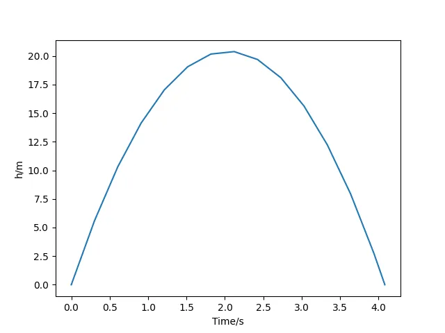
Say, we want to know how long it will take for an apple, launched from the ground into the air, to fall back to the ground. We have the differential equations

\[\begin{split}\left\{ \begin{aligned} &v'=-9.8\\ &h'=v \end{aligned} \right.\end{split}\]

with \(v(0)=20\) and \(h(0)=0\), we can just type the codes

import matplotlib.pyplot as plt
import numpy as np
from Solverz import Model, Var, Ode, Opt, made_numerical, Rodas

# Declare a simulation model
m = Model()
# Declare variables and equations
m.h = Var('h', 0)
m.v = Var('v', 20)
m.f1 = Ode('f1', f=m.v, diff_var=m.h)
m.f2 = Ode('f2', f=-9.8, diff_var=m.v)
# Create the symbolic equation instance and the variable combination 
bball, y0 = m.create_instance()
# Transform symbolic equations to python numerical functions.
nbball = made_numerical(bball, y0, sparse=True)

# Define events, that is,  if the apple hits the ground then the simulation will cease.
def events(t, y):
    value = np.array([y[0]]) 
    isterminal = np.array([1]) 
    direction = np.array([-1]) 
    return value, isterminal, direction

# Solve the DAE
sol = Rodas(nbball,
            np.linspace(0, 30, 100), 
            y0, 
            Opt(event=events))

# Visualize
plt.plot(sol.T, sol.Y['h'][:, 0])
plt.xlabel('Time/s')
plt.ylabel('h/m')
plt.show()

Then we have

The model is solved with the stiffly accurate Rosenbrock type method, but you can also write your own solvers by the generated numerical interfaces. For example, the multidimensional Newton method of AEs is a scheme with formulae

\[y_{k+1} = y_k - J_F(y_k)^{-1}F(y_k)\quad k=0,1,2,\cdots.\]

Its implementation using Solverz can be as simple as

# main loop
while max(abs(df)) > tol:
    ite = ite + 1
    y = y - solve(eqn.J(y, p), df)
    df = eqn.F(y, p)
    if ite >= 100:
        print(f"Cannot converge within 100 iterations. Deviation: {max(abs(df))}!")
        break

The numerical AE object eqn provides the \(F(t,y,p)\) interface and its Jacobian \(J(t,y,p)\), which grants your full flexibility. So that the implementation of the NR solver just resembles the formulae above.

Sometimes you have very complex models and you dont want to re-derive them everytime. With Solverz, you can just use

from Solverz import module_printer

pyprinter = module_printer(bball,
                           y0,
                           'bounceball',
                           jit=True)
pyprinter.render()

to generate an independent python module of your simulation models. You can import them to your .py file by

from bounceball import mdl as nbball, y as y0